
This post is about the method that I use to analyze the New Year addresses. In short, I extract one hundred words that are the most frequent among all of the addresses and then apply correspondence analysis (CA) to their frequencies. People who use CA and similar methods typically don’t discuss in detail how such methods actually work and simply proceed directly to the pretty pictures that those methods produce. However, I believe that every result is more meaningful if we can envision how it was obtained, so I will try to explain how CA works using a simple imaginary example that is straightforward and easy to grasp intuitively.
However, first I tried to come up with a sophisticated story about why a person might need to apply CA. But my ideas were too complicated and unrealistic. One of them, for example, involved a company that suddenly suggested that it would pay for employees’ beverages during the workdays of one week in the summer. An employee found several receipts from various weeks and two frequent buyer cards in her pocket. I tried to use all that information to find out which of these drinks were purchased on workdays during the summer. After concocting this scenario, I decided that it was easier not to try to come up with a realistic backstory and just present a simple illustrative case that’s easy to understand and describes how the method works. Please keep in mind that, even though this case is so straightforward that no one would actually need to use statistical analysis here, it would become much more complicated when more variables are involved, as happens in the case of New Year addresses.

Imagine that Alice found her receipts from Starbucks from a week in January and a week in July. Alice had purchased one drink on each of those days. In the winter it was cold, so she was more interested in hot drinks, whereas in the summer it was hot, and she bought iced coffee and lemonade. Throughout the year, she drank coffee on weekdays on her way to work to jump-start her workday, but at weekends she felt that she did not need to concentrate that much, so she drank tea or lemonade instead of coffee. Table 1 presents the list of the drinks that Alice bought during those two weeks.
Table 1. Drinks that Alice purchased on different days.
| day | day of the week | month | drink |
| 1 | Mon | January | coffee |
| 2 | Tue | January | coffee |
| 3 | Wed | January | coffee |
| 4 | Thu | January | coffee |
| 5 | Fri | January | coffee |
| 6 | Sat | January | hot tea |
| 7 | Sun | January | hot tea |
| 8 | Mon | July | iced coffee |
| 9 | Tue | July | iced coffee |
| 10 | Wed | July | iced coffee |
| 11 | Thu | July | iced coffee |
| 12 | Fri | July | iced coffee |
| 13 | Sat | July | iced lemonade |
| 14 | Sun | July | iced lemonade |
If Alice analyzed her receipts based only on the drinks she had purchased, she would be able to distinguish the receipts from the summer and the receipts from the winter. She would also be able to distinguish the workday receipts from the weekend receipts. Of course, this example is easy to understand so far, but remember that this example will also illustrate how CA works.
First, let’s transform the data in the following way. A new table (Table 2) contains a row for each of the fourteen days for which Alice has receipts. All the words that appear in those receipts – coffee, tea, hot, iced, lemonade – are headings for the columns. Each cell of the table contains a ‘1’ if the word at the top of the column appears in the receipts on that day and ‘0’ if it does not.
We can see that the word coffee can be used to distinguish the workdays and weekends; i.e., every day that contains the word coffee is a workday. The word iced is helpful in determining the month of the receipt; each day that contains the word iced is in July, whereas every day that does not is in January. However, other words are less useful in determining the day of the week and the month. The words tea, hot, and lemonade appear only on weekends; however, none of them appears on all the weekend days in the dataset. Moreover, hot and tea appear exactly on the same days, so if we add information to the model that is contributed by the word tea, then the word hot cannot add any new information to the model.
Table 2. Words that appear in the receipts on different days.
| day | coffee | tea | lemonade | hot | iced |
| 1 | 1 | 0 | 0 | 0 | 0 |
| 2 | 1 | 0 | 0 | 0 | 0 |
| 3 | 1 | 0 | 0 | 0 | 0 |
| 4 | 1 | 0 | 0 | 0 | 0 |
| 5 | 1 | 0 | 0 | 0 | 0 |
| 6 | 0 | 1 | 0 | 1 | 0 |
| 7 | 0 | 1 | 0 | 1 | 0 |
| 8 | 1 | 0 | 0 | 0 | 1 |
| 9 | 1 | 0 | 0 | 0 | 1 |
| 10 | 1 | 0 | 0 | 0 | 1 |
| 11 | 1 | 0 | 0 | 0 | 1 |
| 12 | 1 | 0 | 0 | 0 | 1 |
| 13 | 0 | 0 | 1 | 0 | 1 |
| 14 | 0 | 0 | 1 | 0 | 1 |
Now let’s input Alice’s data to CA. CA reads Table 2 and comprehends it as five points in a 14-dimensional space. For example, coffee became a point with the following fourteen coordinates: (1, 1, 1, 1, 1, 0, 0, 1, 1, 1, 1, 1, 0, 0). Then, CA finds a line to which all five points in the 14-dimensional space are close together. Imagine that if a tube encompassed this line, most or all of the points would be inside the tube. CA proposes that this line is the first new dimension. Then it finds the second line so that the sum of the distances from all the points to the second line and the first line is minimal. CA proceeds similarly until it reaches the number of dimensions in the space, in our case fourteen.
Several first dimensions are the ones that best describe what is happening in the data. They point to the factors that influence the distribution most significantly. In the case study of the receipts, these factors are the days of the week and the seasons. Figure 1 shows the distribution of the fourteen days on the map for the first two dimensions. Days 1 through 5 are grouped together. These are the days when Alice drank non-iced coffee. Days 8 through 12 are also grouped together. These are the days when Alice drank iced coffee. These two groups are located far away from Days 6 and 7 to the right and Days 13 and 15 in the top left corner. On Days 6 and 7, Alice drank hot tea. On Days 13 and 14, Alice drank iced lemonade.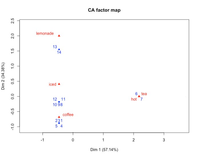 Figure 1. Groups of days according to drinks purchased on that day.
CA thus provides us with more information than could be gleaned from just counting the number of words. From Figure 1 we immediately see that the words hot and tea contribute exactly the same information. We can also observe that lemonade, hot, and tea provide similar information and are located significantly away from coffee. If we were to investigate the information that is contributed only by the words, column by column, we would have to draw these conclusions by ourselves, but CA does this work for us. This capability becomes extremely advantageous when we move from a simple case with a 5 x 14 matrix to a much more complicated case with a larger matrix.
We can map our major factors – days of the week and seasons – as shown in Figure 2. The figure is divided by two lines: purple and green. The purple line separates the seasons; the winter days are below the purple line and the summer days are above the purple line. For this factor, the words iced and lemonade strongly increase the probability of the summer season, whereas the words hot and tea decrease this probability. At the same time, the word coffee appears with the same probability in both the summer receipts and winter receipts, so coffee is not a good predictor for the season factor. The green line separates the workdays, located below the green line, from the weekend days, located above the green line. Here, the word coffee is a strong predictor of the workday, whereas lemonade, hot, and tea strongly predict a weekend day. Here, the word iced is not helpful, because it occurs both on workdays and during the weekend. We can also see that the words tea and hot always appear together, and if we take the information that is provided by the word tea, then the word hot does not add anything to our model. Therefore, one of these words, for example, hot, can be excluded from the analysis.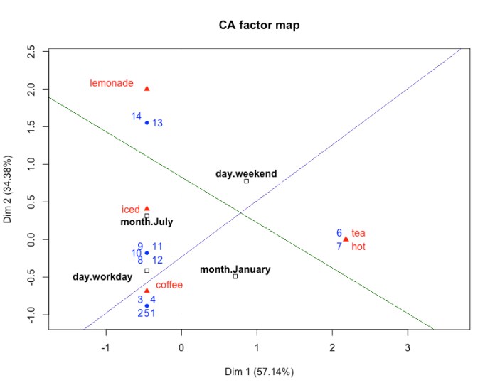 Figure 2. Major factors in a day’s distribution.
In the case of the 100 most frequent words found in the New Year addresses we will have a similar matrix, but a much larger dataset. There will be 100 words instead of 5, and 46 years instead of 14 days. Nonetheless, the underlying idea is similar. I analyzed the matrix using words as the headings of the rows and years as the headings of the columns. Each cell of the matrix contained the frequency of the word in the New Year address given that year, measured in items per million (ipm). Items per million is traditionally used in corpus linguistics as a measure of frequency that does not depend on the size of the document. For example, the word bol’šoj ‘big’ appears three times in the New Year address delivered in 1970. The length of the New Year address that year was 605 words. Therefore, in the cell at the intersection of the row for the word bol’šoj ‘big’ and the column for 1970, we have 4958.68 = (3/605) * 1,000,000. Measuring the frequency of words in ipm is necessary because the lengths of the addresses vary notably – from 1445 words in 1993 to 194 words in 2012.
Unfortunately, unlike in the simplified case of Alice’s Starbucks receipts where the main factors, seasons and workdays versus weekends, are already known to us, in the case of the New Year addresses, we do not know the main factors that contribute to the distribution. In the following posts I will investigate the important dimensions for the New Year addresses and interpret those dimensions. For each dimension, I will show what it correlates with in the real world. I will start with the most important dimension – the political system – in the next post.

Pingback: Dimension 1: Political era | Reading the data leaves